

MLB Betting Models: A Builder’s Guide for 2026
An MLB betting model is a probabilistic prediction system that converts game-level inputs into calibrated probabilities across moneyline, run line, totals, and player prop markets. The core value is straightforward: when your model’s probability for a given outcome exceeds the implied probability embedded in the sportsbook’s line, a positive expected value (+EV) bet exists. That edge, compounded across many games in a full MLB season, is what separates disciplined model-based wagering from guesswork.
Here is what a working MLB prediction model produces:
- Core outputs: Win probability per team, full run distribution, P(Over) for totals, run-line margins, and selected prop probabilities such as NRFI (no run first inning) and strikeout totals
- Key inputs: Starting pitcher metrics, projected lineup, park factors, weather conditions, and Statcast pitch-level features
- Practical uses: Identify +EV bets, size stakes using Kelly or flat units, and line-shop across multiple sportsbooks to maximize the value of each edge
Pro Tip: Start with one market, moneyline or NRFI, and prove a live edge using walk-forward backtests before expanding to run lines, totals, or props. Spreading across markets too early dilutes your ability to diagnose what is and is not working.
Table of Contents
- What do MLB betting models actually predict?
- Which model architecture should you use?
- What data and features do MLB models need?
- How do you build an MLB model from scratch?
- How do you evaluate model quality and backtest results?
- How do you turn model probabilities into real bets?
- How does the right model change by bet type?
- What tools and data feeds do you actually need?
- What does a recommended production baseline look like?
- Model limitations and responsible gambling
- Key Takeaways
- Why model discipline matters more than model complexity
- Mannysvariety delivers verified MLB picks without the pipeline burden
- Useful sources and further reading
What do MLB betting models actually predict?
The output of a well-built model is not a pick. It is a probability. For a moneyline market, the model assigns each team a win probability, say 58% for the home team. The sportsbook’s line implies its own probability, which you extract by designing the posted odds. If the book’s de-vigged implied probability is 52%, the edge is 6 percentage points.
The EV calculation is direct. For a $100 bet at American odds of -110 (decimal 1.909):
EV = (p × payout) − (1 − p) × stake EV = (0.58 × $90.91) − (0.42 × $100) = $52.73 − $42.00 = +$10.73
A positive EV does not guarantee a win on any single bet. It means the bet is priced in your favor, and over a large sample, positive EV bets produce profit.
Calibration is what makes or breaks this math. An overconfident model that assigns 70% win probability to a team that actually wins 55% of the time will generate misleading EV signals and lead to poor stake sizing. One practitioner project reduced its maximum calibration gap from roughly 42% to approximately 3.2% by layering a Monte Carlo simulator over a hierarchical Bayesian skill model, producing run distributions that matched realized outcomes far more tightly than a single-stage regressor.
Calibration check: A model that says “70% confidence” should be right about 70% of the time across all bets it rates at that level. If it is right only 55% of the time at that threshold, the model is overconfident and your sizing will be wrong.
Which model architecture should you use?
Research comparing multiple ML approaches confirms there is no single best architecture. The right choice depends on your priorities: interpretability, raw performance, or coherent probability outputs across correlated markets.
- Logistic regression: High interpretability, fast to train, easy to audit. Coefficients map directly to feature importance. Best for beginners or any context where you need to explain every prediction. Limited capacity means it will underlit complex non-linear relationships.
- XGBoost / LightGBM: The practical production standard for MLB prediction models. Gradient-boosted trees handle missing values, non-linear interactions, and mixed feature types without heavy preprocessing. LightGBM trains faster than XGBoost on large datasets and often matches or exceeds it on tabular sports data. Both require careful hyperparameter tuning and temporal validation to avoid overfitting.
- Neural networks: Flexible and capable of learning subtle pitch-sequence patterns or batter-pitcher interaction effects. Data-hungry and harder to debug. Best suited for fine-grained prop models or hybrid stacks where you have several seasons of pitch-level Statcast data.
- Hierarchical Bayesian / probabilistic simulators: The strongest choice when you need coherent probabilities across correlated markets (moneyline, run line, and totals must be internally consistent). A Bayesian skill model feeding a per-plate-appearance Monte Carlo simulator enforces that consistency and quantifies uncertainty explicitly.
- Ensembles: Combining LightGBM outputs with a Bayesian simulator or a logistic regression meta-learner typically reduces variance and improves calibration. The tradeoff is added complexity in maintenance and debugging.
For most builders, the practical path is: start with logistic regression to understand your features, graduate to LightGBM as your production baseline, and layer in a simulator once you need coherent multi-market outputs.

What data and features do MLB models need?
The quality of your features determines the ceiling of your model. Raw box scores are a starting point, not a finish line.
Primary data sources:
- Baseball Savant: Statcast-derived metrics including spin rate, exit velocity, launch angle, expected batting average (xBA), and expected weighted on-base average (xwOBA). The best free source for pitch-level data.
- FanGraphs: Advanced batting and pitching rate stats: FIP, xFIP, SIERA, wRC+, and Barrel%. Leaderboards are easy to scrape or export.
- Retrosheet: Historical play-by-play and boxscore data going back decades. Indispensable for building long training windows and validating park factors.
- Paid API feeds: Worth the cost once you need guaranteed daily delivery and low-latency lineup data. Free sources work fine for prototyping.
Features that consistently add predictive signal:
Pitcher vs. batter platoon splits (left/right matchups), rolling 7/30/90-day rate stats weighted by innings pitched or plate appearances, projected batting order position, bullpen leverage index and days-of-rest fatigue, park run factors by handedness, umpire strike-zone tendencies, temperature and wind direction at first pitch, and day/night game adjustments.
Feature engineering notes: Use IP-weighted rolling metrics rather than simple averages to prevent a single dominant start from distorting a pitcher’s recent form. One-hot encode categorical fields like park ID and umpire. Build fallback rules for missing lineup data (common with late scratches) so your pipeline does not break on game day. For simulators, per-plate-appearance or per-inning features are more useful than game-level aggregates because the simulator needs granular event probabilities to generate realistic run distributions.
How do you build an MLB model from scratch?
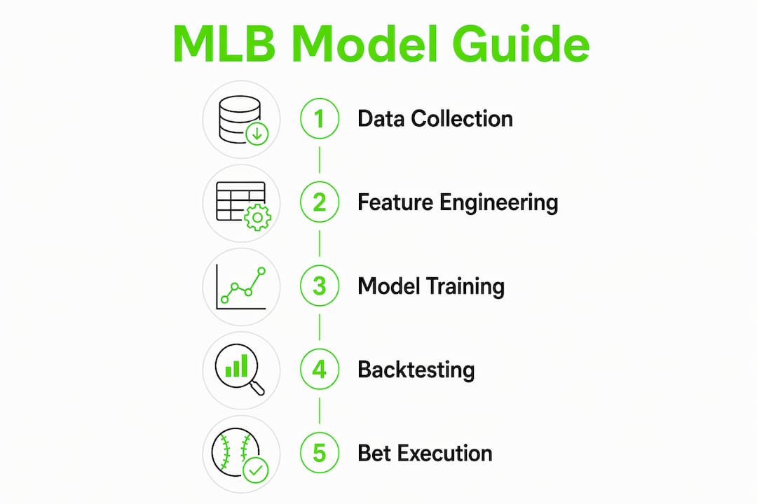
A working pipeline has eight ordered steps. Skipping any one of them creates a gap that will surface as unexplained variance or inflated backtested returns.
- Data ingestion and cleaning: Pull from Baseball Savant, FanGraphs, and Retrosheet. Standardize player IDs across sources. Flag and handle missing values explicitly.
- Feature engineering and lineage: Build your feature set with documented transformations. Store raw data separately from derived features so you can recompute from scratch.
- Time-aware train/validation split: Never use future data to train a model that will predict past games. Split chronologically: train on seasons 1 through N-1, validate on season N.
- Model training and hyperparameter tuning: Use cross-validation within the training window only. Tune on a held-out validation fold, not the test set.
- Calibration: Apply isotonic calibration or Platt scaling trained on out-of-fold predictions. This step aligns predicted probabilities with realized frequencies and is non-negotiable for accurate EV calculations.
- Production inference and journaling: Log every prediction at the time it is generated: model version, input features, raw probability, de-vigged implied probability, edge at posting time, and final outcome.
- Automation: Schedule a morning sync to pull the previous day’s final data, fetch today’s confirmed lineups and starting pitchers, and generate predictions before lines move.
- Weekly retrain and end-of-season evaluation: Retrain on a rolling window weekly. At season’s end, run a full self-evaluation against the predictions journal.
Common pitfalls to avoid:
- Data leakage from features derived using future information (e.g., a season-level ERA that includes the game being predicted)
- Overfitting on a single season’s worth of data (use at least four to six seasons for training)
- Ignoring late lineup changes and starting pitcher scratches
- Comparing model probabilities directly to posted odds without de-vigging first
Pro Tip: An append-only predictions journal is the single most important operational habit. Store model version, inputs, raw probabilities, implied edge at posting time, and the final outcome. Without it, you cannot honestly grade your model or detect when it has drifted.
The mlb-bet-engine project implements walk-forward backtests from 2014 onward with exactly this kind of append-only journal and automated end-of-season self-evaluation, making it a useful reference for pipeline structure.
How do you evaluate model quality and backtest results?
Backtested accuracy is the most misread number in sports betting analytics. A model that shows 65% accuracy on historical data can drop to roughly 51% in live betting due to overfitting and distribution shift. Walk-forward backtesting, where each validation window is strictly after its training window, is the primary defense against this gap.
Metrics that matter:
| Metric | What it measures | Target |
|---|---|---|
| Brier score | Mean squared error of probabilities; lower is better | — |
| Log loss | Penalizes confident wrong predictions heavily | — |
| ROI / CLV | Economic return; closing line value as a proxy for edge | Positive over 500+ bets |
| Calibration plot | Predicted vs. realized win rates by probability bucket | Diagonal alignment |
| ROC/AUC | Discriminative ability across thresholds | — |
Backtesting checklist:
- Use only information available at the time of the prediction (posting-time lineups, not final lineups)
- De-vig sportsbook odds before computing implied probabilities and edge
- Evaluate across multiple seasons, not just one favorable stretch
- Slice results by market type (day vs. night, home vs. away, first-5 innings vs. full game)
- Test multiple probability cutoff thresholds before settling on a betting threshold
Statistical warning: Betting every game a model rates is almost always a losing strategy. Academic analysis shows that applying probability cutoffs, abstaining on close games where the model’s edge is thin, can turn a losing naive strategy into a positive-return one. Selective flagging is not cherry-picking; it is proper threshold optimization.
How do you turn model probabilities into real bets?
The workflow from model output to placed bet has four steps, and each one affects your long-run results.
- De-vig the sportsbook line. Convert American odds to implied probabilities, then remove the vig (overround) to get the book’s fair-odds estimate. A common method is the multiplicative method: divide each raw implied probability by their sum.
- Compare model probability to de-vigged implied probability. If your model says 58% and the book’s de-vigged probability is 52%, the edge is 6 percentage points.
- Calculate EV. Use the formula from the opening section. Only bet when EV is positive and the edge clears your minimum threshold (typically 3–5% after accounting for variance).
- Size the bet. Three approaches, in order of aggressiveness:
- Flat units: Bet the same unit size on every qualifying bet. Simple, low variance, easy to track. Best for beginners.
- Fractional Kelly: Kelly criterion calculates the theoretically optimal bet size as edge / odds. Quarter Kelly (25% of full Kelly) is the most common production setting. It reduces variance significantly while preserving most of the long-run growth.
- Full Kelly: Maximizes long-run bankroll growth but produces extreme variance. Not recommended unless your model’s calibration is verified over thousands of bets.
Pro Tip: Always line-shop across multiple sportsbooks before placing a bet. A 2% difference in odds compounds materially over a full season. Log the odds at posting time in your predictions journal, not the odds you eventually got, to avoid hindsight bias when grading.
Line shopping across books is one of the highest-leverage habits a model-based bettor can build. Even a small consistent price improvement changes break-even thresholds meaningfully over 500 or more bets.
How does the right model change by bet type?
Different markets require different modeling approaches and data inputs. A moneyline model and a strikeout prop model share some features but diverge sharply in what drives accuracy.

| Bet type | Primary modeling approach | Key data required |
|---|---|---|
| Moneyline | Run-distribution simulator or ML classifier | Starter ERA/FIP, bullpen depth, lineup wRC+, park factor |
| Run line | Coherent joint simulation (home/away correlated) | Full run distribution, starter quality, bullpen leverage |
| Totals (O/U) | Run-distribution model or totals classifier | Park run factor, weather/temp, starter K-rate, bullpen ERA |
| NRFI / F5 | Starter-isolated model | Starter xFIP, recent form, opposing lineup splits |
| Strikeout props | Player-event model | Pitcher K%, opposing K%, umpire zone size, pitch mix |
| Same-game parlays | Correlated joint simulator | All of the above; correlation structure across outcomes |
Run-line modeling specifically benefits from a coherent joint simulation. If you model home and away run totals independently, you can produce combinations that violate basic probability constraints (e.g., the model implies the home team wins by 2 more often than the run distribution supports). A correlated Monte Carlo simulator prevents that.
For NRFI and first-5-innings markets, isolating starting-pitcher effects reduces bullpen noise and makes the market more modelable. Practitioner write-ups consistently flag these markets as higher-ROI targets when a model has strong starter-quality features.
The FTN Fantasy SGP correlation tool demonstrates how joint-simulation logic applies to same-game parlays: it estimates how frequently selected outcomes coexist across many simulated games, which is exactly the kind of correlation structure a production model needs to price SGPs accurately.
What tools and data feeds do you actually need?
You do not need a paid data subscription to build a prototype. Free sources cover the essentials. Paid feeds become worth it once you need reliability and sub-hour latency for daily lineup updates.
Free sources:
- Baseball Savant / Statcast: Pitch-level data, Statcast metrics, and game-level summaries. The primary free source for advanced MLB stats.
- FanGraphs: Rate stats, leaderboards, and projections. Exportable CSVs for most tables.
- Retrosheet: Historical play-by-play going back to the 1950s. Essential for long training windows.
Local data storage:
- DuckDB: Fast, serverless analytical database. Ideal for local warehousing of Statcast and FanGraphs exports without standing up a full Postgres instance.
- Postgres: Better for production pipelines with multiple data sources and concurrent reads.
ML libraries:
- LightGBM / XGBoost: Gradient-boosted tree frameworks. Both have Python APIs and integrate cleanly with scikit-learn pipelines.
- scikit-learn: Preprocessing, calibration (isotonic and Platt), and model evaluation utilities.
- NumPyro / JAX: Probabilistic programming for Bayesian models and Monte Carlo simulators.
Automation:
Schedule a morning sync job to pull the previous day’s final Statcast data and today’s confirmed lineups. Run a weekly retrain with a validation gate. If recent moneyline accuracy regresses more than 2 percentage points versus the prior model version, the automated rollback logic restores the previous model automatically, a guardrail that prevents a bad retrain from going live.
What does a recommended production baseline look like?
The baseline that balances speed, reproducibility, and strong out-of-sample performance in practitioner projects follows a two-stage architecture.
Stage A: LightGBM regressors predict expected runs per team using pitcher, lineup, park, and weather features. A six-year rolling training window with weekly retrains and a 14-day validation gate keeps the model current without overfitting to recent noise.
Stage B: A correlated Monte Carlo simulator takes Stage A’s expected-run outputs and generates a full joint run distribution across thousands of simulated games. From that distribution, the pipeline derives coherent moneyline, run-line, and over/under probabilities. Isotonic calibrators trained on out-of-fold predictions are applied at the end to align predicted probabilities with realized frequencies.
This architecture matches the production design described in the Rene Nunez MLB project, which reduced its maximum calibration gap from roughly 42% to approximately 3.2% using this two-stage approach.
Pro Tip: Run a full end-of-season self-evaluation every October. Compare your model’s predicted probabilities against realized outcomes using a calibration plot and Brier score. If calibration has drifted, retrain the calibrator before the next season starts.
Similar discipline applies in other performance-evaluation contexts. The same principles that govern prop trading account evaluation, strict out-of-sample grading, documented methodology, and rollback triggers, translate directly to model-based sports betting.
Model limitations and responsible gambling
Even a well-calibrated model with a verified edge will lose a large share of individual bets. MLB variance is high. A team with a 60% win probability loses 40% of the time by definition, and losing streaks of 10 or more bets are statistically normal. Expecting consistent short-run profits from any model is a misunderstanding of probability, not a model failure.
Markets are also partially efficient. Sharp bettors and professional syndicates move lines quickly. Large, obvious edges get priced out within minutes of opening. The edges that survive to game time tend to be smaller and more situational, which is why selectivity and threshold optimization matter so much.
Bankroll management rules:
- Bet 1–3% of your total bankroll per unit on flat staking
- Use quarter Kelly (25% of full Kelly) as a ceiling for any single bet
- Set a daily or weekly loss cap and stop betting when you hit it
- Never chase losses by increasing unit size
Model outputs are predictive tools, not guaranteed income. Obey your state’s sports betting laws. Regulations vary by jurisdiction across the United States, and betting in a state where it is not legally authorized carries legal risk regardless of model quality.
This article is general information, not legal or financial advice. Confirm current regulations with your state’s gaming authority or a qualified professional before wagering.
Key Takeaways
A production-ready MLB betting model requires calibrated probabilities, walk-forward backtesting, and disciplined staking to generate consistent positive expected value over a full season.
| Point | Details |
|---|---|
| Start with one market | Prove edge on moneyline or NRFI with walk-forward backtests before expanding to other markets. |
| Calibration is non-negotiable | Apply isotonic calibration on out-of-fold predictions; uncalibrated probabilities produce wrong EV signals and poor sizing. |
| De-vig and log at posting time | Always de-vig sportsbook odds and record them at posting time to avoid hindsight bias when grading. |
| Use fractional Kelly or flat units | Quarter Kelly caps variance while preserving long-run growth; flat units are simpler and safer for new builders. |
| Mannysvariety as a turnkey option | For bettors who want verified, production-ready MLB picks without building a pipeline, Mannysvariety provides audited picks with a transparent track record. |
Why model discipline matters more than model complexity
The conventional wisdom in sports betting analytics fixates on algorithm selection: which model architecture wins? The more important question is whether the pipeline around the model is honest. A logistic regression with walk-forward validation, isotonic calibration, and an append-only predictions journal will outperform a neural network trained on the full dataset and graded with hindsight.
What most guides understate is the gap between backtested and live performance. Backtested accuracy of 65% dropping to roughly 51% in live conditions is not an edge case; it is the norm for models built without strict temporal splits. The model looks good on paper because it has seen the future during training. Walk-forward backtesting closes that gap, but it requires discipline to implement correctly and patience to accept that the resulting numbers will be less impressive than the naive version.
The other underappreciated point: selectivity is a feature, not a workaround. Abstaining on games where your model’s edge is thin is not cherry-picking results. It is threshold optimization, and it is what separates a model that generates positive returns from one that bleeds units on every close game. The research on probability cutoffs makes this explicit: naive betting on every game loses money; selective betting above a calibrated threshold can produce positive returns.
Build the pipeline right. Grade it honestly. The model complexity can come later.
Mannysvariety delivers verified MLB picks without the pipeline burden
Building a production MLB model takes months of data engineering, calibration work, and live grading before you know whether it has a real edge. Mannysvariety removes that infrastructure entirely. The platform’s sport-specific AI engine runs thousands of simulations daily, producing MLB picks, player props, and parlays with a publicly tracked win rate of 63.5% across more than 1,600 graded picks and a net return of 443.9 units.

Every pick is archived permanently, so the performance record is verifiable, not self-reported. Daily reports include market analysis, prop predictions, and lineup-aware picks delivered before lines move. For bettors who want to apply data-driven baseball betting strategies without building and maintaining their own model, Mannysvariety’s Atlas predictive engine provides the production-ready output directly.
Subscription tiers include a free trial with limited features, short-term day and week passes, and full Core and Elite plans. Check current pricing and plan details to find the option that fits your betting volume and budget.
Useful sources and further reading
- Baseball Savant / Statcast: Official MLB Statcast data portal. Pitch-level metrics, game logs, and leaderboards. Free.
- FanGraphs: Advanced rate stats, projections, and leaderboards. Free tier covers most modeling needs.
- Retrosheet: Historical play-by-play data. Essential for multi-season training windows.
- ShamgarBN/mlb-bet-engine (GitHub): Open-source production pipeline with walk-forward backtests from 2014, append-only predictions journal, automated morning sync, weekly retrain, and rollback logic. Strong reference for pipeline architecture.
- Rene Nunez MLB Model Project: Two-stage hierarchical Bayesian + Monte Carlo simulator with documented calibration results. Useful for understanding coherent multi-market probability derivation.
- arXiv: Assessing win strength in MLB win prediction models: Academic comparison of ML architectures for MLB win prediction, including analysis of probability cutoff optimization.
- FTN Fantasy Betting Tools: SGP correlation tool and joint-simulation resources for same-game parlay modeling.
Reproducibility note: Prefer projects that publish prediction journals, open-source code, and documented backtests. A model without a verifiable grading record is a marketing claim, not a production tool. End-of-season self-evaluation reports, comparing predicted probabilities to realized outcomes via calibration plots and Brier scores, are the gold standard for honest model assessment.