

Monte Carlo Betting: A Bankroll Risk Guide for Bettors
Monte Carlo betting uses repeated randomized simulations to show the range of possible bankroll outcomes from a given staking plan. Instead of guessing whether your edge and unit size will hold up, you run the plan thousands of times against randomized outcomes and see the spread: median return, worst-case drawdown, and the probability that you go broke before the edge pays off.
Use it any time you want to stress-test a staking plan before real money is on the line. Bettors reach for Monte Carlo simulations to size units against a known or estimated edge, compare how different sportsbooks’ odds affect long-run outcomes, and set stop-loss thresholds before variance does the deciding for them.
The practical verdict, in three moves:
- Run at least 10,000 simulated bankroll paths before committing serious money to any staking plan.
- Use the 5th percentile outcome, not the average, to size your units and set a stop-loss.
- Re-run the simulation any time your win rate, odds, or bankroll target changes materially.
Pro Tip: If you only take one number away from a simulation, make it the probability of ruin. A staking plan with a great median return but a significant chance of busting your bankroll is not a good plan.
Key Takeaways
Monte Carlo simulation turns a staking plan from a guess into a measurable set of outcomes, and the probability of ruin matters more than the average return when deciding whether to actually use it.
| Point | Details |
|---|---|
| Simulate before you stake | Run at least 10,000 trials to get stable percentile and ruin estimates before committing real bankroll. |
| Trust percentiles over averages | Use the 5th percentile outcome, not the mean, to size units and set stop-loss thresholds. |
| Watch drawdown, not just growth | A high median return paired with a deep max drawdown can still be a bad plan for risk-averse bettors. |
| Model correlation explicitly | Same-game parlays and same-day multiples aren’t independent bets, and treating them that way understates risk. |
| Automate the analysis | Mannysvariety applies simulation-informed sizing and reporting across its AI-driven pick engines for readers who want this analysis done for them. |
Table of Contents
- What Monte Carlo Betting Actually Simulates
- Why Bettors Run These Simulations In The First Place
- Inputs And Assumptions You Need Before You Simulate
- How To Run A Monte Carlo Simulation Step By Step
- Reading Your Results: EV, Percentiles, And Risk Of Ruin
- Two Worked Examples You Can Reproduce
- Picking The Right Tool For Your Simulation
- Where Monte Carlo Models Go Wrong
- Turning Simulation Output Into A Staking Plan
- Backtesting And Monte Carlo Work Better Together
- The Blind Spot Most Bettors Don’t See Coming
- Get Simulation-Backed Picks Instead Of Building Your Own Model
- Frequently Asked Questions
- Sources
What Monte Carlo Betting Actually Simulates
A Monte Carlo simulation is repeated random sampling used to map a distribution of possible futures rather than produce one forecast. You feed it your bankroll, your edge, your bet size, and your odds. It then draws random win/loss outcomes for each simulated bet, thousands of times over, and records where your bankroll ends up in each run. The output isn’t a prediction. It’s a shape: a curve showing how often you’d end up broke, break even, doubled, or somewhere in between if reality played out the way your inputs assume it would.

This is fundamentally different from trying to predict a single outcome, and it’s also different from a much more common (and costly) way bettors think about randomness: the gambler’s fallacy. That’s the mistaken belief that independent random events are somehow “due” to balance out, like assuming a coin is more likely to land tails after five straight heads, as Wikipedia’s overview of the fallacy explains. Monte Carlo simulation does not correct for streaks or “even things out.” Each simulated bet is drawn independently, exactly like the real bets it’s modeling. The value isn’t in predicting when your luck turns. It’s in showing you what a large number of independent, unpredictable outcomes does to a bankroll over time.
Picture a simple coin-flip example. Flip that virtual coin 500 times, in one simulated run, and you might end up nicely ahead. Run it again with a fresh set of 500 random flips and you might be down 20 units at some point during the run, even though your long-run edge hasn’t changed at all.
That’s what separates a real analysis from wishful thinking. A few concepts do the heavy lifting here:
- Expected value (EV): what you’d earn per bet on average, given your edge and odds.
- Variance: how much individual outcomes swing away from that average.
- Percentiles: where your bankroll lands at specific points in the outcome distribution (the bottom 5%, the top 95%, and everything between).
- Risk of ruin: the share of simulated runs where your bankroll hits zero before your edge has time to play out.
A Monte Carlo simulation doesn’t tell you what will happen. It tells you, with real numbers, what a whole population of equally likely futures looks like, so you can plan for the bad ones instead of hoping they don’t come.
Why Bettors Run These Simulations In The First Place
Monte Carlo simulation earns its place in a bettor’s toolkit because it answers questions that gut instinct and spreadsheets full of past results can’t. According to SportsBetEdge’s breakdown of the method, professionals use it specifically for bet sizing and for finding value against the closing line, not for picking winners.
The questions it’s built to answer are concrete:
- Will my bankroll survive a 12 game losing streak at my current unit size?
- What’s my realistic probability of going broke before my edge materializes over a full season?
- What does my bankroll look like after 500 bets, not just on average, but across the worst 5% of outcomes?
- How much wider is my outcome spread if I bet 3% of bankroll per play instead of 1%?
These aren’t abstract questions. They drive real decisions. A bettor comparing flat staking against a percentage-of-bankroll model can run both through identical simulated bet sequences and see, side by side, which one produces a survivable drawdown at the same long-run growth rate. A bettor deciding between two sportsbooks offering slightly different odds on the same market can simulate both odds sets against the same assumed win rate and see how much that half-point of vig actually costs over a season, not just per bet.
Simulations also drive stop-loss design. That number is defensible. A gut-feel stop-loss usually isn’t.
None of this requires you to know the future. It requires you to be honest about your edge and your variance, then let the simulation show you the consequences of both.
Inputs And Assumptions You Need Before You Simulate
The quality of a Monte Carlo betting model depends entirely on what you feed it. Garbage inputs produce a confident-looking, completely useless output. Before running anything, you need to nail down a specific list of inputs and be explicit about the assumptions baked into each one.
Core inputs:
- Starting bankroll: the actual dollar (or unit) amount you’re modeling.
- Bet sizing rule: flat units, full or fractional Kelly, or a fixed percentage of current bankroll.
- Number of bets: how many wagers the simulation should run per path (a season, a month, 1,000 bets).
- Odds: either a single average price or a realistic distribution if your bets span a range of markets.
- Estimated true win probability: your actual edge, not the implied probability from the odds alone.
- Fees and commission: relevant for exchange betting or markets with a built-in vig you want to isolate.
Assumptions that quietly decide your results:
- Whether bets are independent or correlated (same-game parlays and same-day multiple bets on one team are rarely independent).
- Whether your win rate is stationary across the whole simulated period or degrades as books adjust to your action.
- Whether the odds you’re modeling reflect one static number or the real variability you’d face across a season of line shopping.
- Whether the sportsbook enforces stake caps or limits that would prevent you from actually placing your modeled bet size.
- Whether you, the bettor, would realistically change your stake mid-streak, which most static models don’t account for.
A quick data hygiene checklist before you trust any output: confirm your odds source reflects what you’d actually get (not a theoretical no-vig line), make sure your win-rate estimate comes from a sample large enough to mean something (a 20-bet hot streak is not a win rate), and decide upfront how you’ll handle inconsistent or missing historical data rather than quietly excluding the bets that don’t fit your story.
How To Run A Monte Carlo Simulation Step By Step
The algorithm behind every betting Monte Carlo simulation, whether you build it in Excel, Python, or an online calculator, follows the same basic shape. SportsBetEdge frames the core steps as defining a probability distribution, sampling from it repeatedly, and aggregating the results, and that structure holds regardless of the tool.
- Set your inputs. Starting bankroll, bet size rule, number of bets per simulated path, odds, and estimated win probability.
- Draw a random outcome for each bet. Generate a random number, compare it against your win probability, and mark the bet win or loss accordingly.
- Apply your staking rule. Adjust the bankroll up or down based on the bet’s size and the odds, using whatever staking method you’re testing.
- Update the running bankroll total and record it, along with whether the bankroll has dropped to zero (ruin) at any point.
- Repeat for the full number of bets in that path, then repeat the entire path thousands of times to build a distribution of outcomes.
The number of simulated paths (M) and bets per path (N) both matter more than most people assume. A handful of the platforms built specifically for this, including BetToolKit’s simulator, recommend running 10,000 or more full simulations to get tail-risk estimates you can actually trust. Fewer than that and your 5th percentile estimate can shift noticeably every time you rerun it, which tells you the sample size isn’t stable yet.
On the technical side, random number generation, seeding, and reproducibility deserve attention too. If you’re building this yourself, set a fixed random seed while you’re testing so you can rerun the exact same simulation and confirm your code changes didn’t silently break anything, then remove the seed (or vary it) once you want fresh randomized outcomes for your actual analysis.
Implementation options, by tool:
- Excel: Build it with
RAND()for outcome draws,IF()statements to apply your win threshold, and a Data Table to run multiple iterations at once, an approach Excel’s built-in statistical functions support natively, per Microsoft’s product overview. - Python: Use
numpy.randomto generate outcome draws at scale andpandasto store and analyze the resulting bankroll paths, an approach backed by Python’s broader scientific ecosystem. - R: Comparable to Python, using base R’s random sampling functions plus vectorized operations for speed across large numbers of trials.
- Online calculators: Tools built specifically for betting simulations, useful for a quick sanity check without writing any code.
Pro Tip: Run the same simulation setup three or four times with different random seeds before you trust the percentile numbers. If your 5th percentile outcome swings wildly between runs, you haven’t run enough trials yet.
Reading Your Results: EV, Percentiles, And Risk Of Ruin
A finished Monte Carlo simulation hands you a wall of numbers. Knowing which ones actually matter for a staking decision is where most of the value lives.
Median versus mean is the first distinction worth internalizing. Betting outcomes are typically skewed, meaning a small number of huge winning runs can drag the average (mean) outcome up while most simulated paths land somewhere lower. The median, the outcome right in the middle of all your simulated paths, tends to give a more honest picture of what a “typical” outcome actually looks like. If your mean and median are far apart, that gap itself is telling you something about how lopsided your outcome distribution is.
Percentiles turn that distribution into decision-ready numbers. The 5th percentile shows you a genuinely bad but plausible outcome. The 95th shows you a genuinely good one. Sportsbook simulation tools generally treat these percentile bands, along with maximum drawdown, as more actionable for bettors than a single average figure, because they show the actual spread you need to survive, not just the destination you’re hoping for.
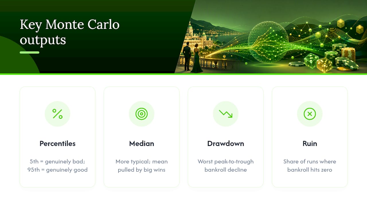
Maximum drawdown measures the worst peak-to-trough decline your bankroll experiences during a simulated run, and academic work on drawdown statistics provides the estimation techniques most simulators build on for measuring this kind of tail risk in randomly generated paths. Probability of ruin is the share of all your simulated paths where the bankroll hits zero before the run ends.
Here’s what typical outputs look like, and what each pattern implies for a bettor deciding whether to actually deploy a staking plan:
A high median paired with a brutal 5th percentile and a double-digit probability of ruin is a red flag for anyone who can’t afford to actually lose the money. That plan might work great on average and still be wrong for you.
Sizing is almost always the fastest fix.*
Two Worked Examples You Can Reproduce
Numbers only mean something once you can rebuild them yourself. Here are two setups, one for sports betting and one for a casino game, with every input listed so you can run either one in Excel or Python and land close to the same outputs.
Example A: A sports betting series with flat units versus fractional Kelly
Quarter Kelly produces a higher median and a wider upside, but it also produces a deeper typical drawdown and a slightly higher ruin probability, because bet sizes grow with the bankroll during winning stretches and shrink during losing ones, amplifying both directions. A bettor who can’t tolerate that should stick with flat staking, even though the math says Kelly grows the bankroll faster on average.

Example B: A roulette even-money color bet
Unlike the sports betting example, this one has a negative expected value baked into every single spin, and the simulation shows it clearly: the median outcome is a loss, not a gain, and nearly one in five simulated paths ends in ruin. Casino simulators consistently flag that progressive staking systems like Martingale look tempting in short simulated windows but produce catastrophic ruin probabilities once you extend the run length, since a long enough sequence eventually generates a losing streak no doubling scheme can survive, per independent Monte Carlo simulator analysis. No staking rule fixes a negative edge. Simulation just makes that fact impossible to ignore.
To reproduce either example in Excel: generate a random number per row with RAND(), flag it a win if it’s below your win probability, calculate bankroll change based on your odds and stake, then use a Data Table with the number of simulations as your input variable to run thousands of full paths at once.
Picking The Right Tool For Your Simulation
Your choice of tool should match your technical comfort and how large a simulation you actually need to run.
- Online calculators work well for a fast sanity check on a single staking question, no setup required, though most cap how many trials you can run or how much you can customize the odds distribution.
- Excel templates hit a strong middle ground: accessible to anyone comfortable with spreadsheets, fully reproducible, and transparent enough that you can see exactly how every number was generated. The tradeoff is speed once you push past a few thousand trials.
- Python or R scale to tens of thousands of trials in seconds and let you model correlated bets, variable odds distributions, and custom staking rules that spreadsheets struggle to handle cleanly.
Whatever you pick, check it can actually do what you need: set a realistic odds distribution rather than one fixed number, model correlation between bets (critical for parlay legs that share an underlying game or player), apply your chosen staking rule automatically bet over bet, export percentile data rather than just an average, and run at least 10,000 trials without choking. Once you’re testing multiple staking rules across multiple sports, Python earns its keep.
Where Monte Carlo Models Go Wrong
A Monte Carlo simulation is only as trustworthy as the assumptions inside it, and a few mistakes show up constantly.
- Using an unreliable win-rate estimate. A 55% win rate calculated from 30 bets is closer to noise than a real edge, and feeding it into a simulation just launders that noise into official-looking numbers.
- Ignoring correlation between bets. Same-game parlays, same-day doubles on one team, or props tied to a single player’s usage all move together, and treating them as independent understates your real variance badly.
- Running too few trials. Anything under a few thousand simulated paths leaves your tail estimates (the 5th percentile, probability of ruin) unstable and unreliable.
- Confusing simulation output with a guarantee. A 96% chance of avoiding ruin still means a 4% chance you don’t, and that 4% still happens to real people.
- Overfitting to historical sequences. Calibrating a model too tightly to a specific stretch of past results, and mistaking that stretch’s quirks for a repeatable edge, produces confident numbers built on a coincidence.
- Ignoring sportsbook limits. A simulation that assumes unlimited stake sizes doesn’t match a market where books cap or limit sharp bettors once you win consistently.
The fix for most of these is the same: run a sensitivity analysis by varying your win-rate estimate up and down a couple of points and see how much your ruin probability moves. If a small change in your edge estimate swings the outcome from safe to dangerous, your model is more fragile than it looks, and a conservative edge estimate protects you better than an optimistic one ever will.
Turning Simulation Output Into A Staking Plan
The entire point of running these numbers is to make a specific staking decision, not to admire a chart.
- Check your probability of ruin first. If it’s above the level you can tolerate, cut your bet size before you touch anything else about the strategy.
- Compare drawdown tolerance against your staking rule. Flat staking produces steadier, more predictable drawdowns; fractional Kelly produces faster growth on average but wider swings, so match the rule to how much variance you can actually stomach watching happen to real money.
- Pick your Kelly fraction based on the simulated tradeoff, not a formula alone; exploring how to understand poker strategy can deepen your grasp of this decision. Full Kelly maximizes long-run growth mathematically but produces brutal drawdowns in simulation. Half Kelly cuts growth modestly while cutting drawdown severity substantially. Quarter Kelly trades more growth for a notably smoother ride, which is why most disciplined bettors who use Kelly at all use a fraction of it, not the full formula.
- Set your timeframe expectations using the percentile spread, not the median alone. Over a short run of 50 or 100 bets, even a real edge can look invisible inside the noise. Over 500 or 1,000 bets, the median outcome starts converging toward what your actual edge and odds predict.
If line movement is a factor in how you shop for odds, build that variability into your input distribution rather than assuming one fixed price across the whole simulated season. A staking plan that looks safe at -110 can look considerably riskier once you account for the worse prices you’ll sometimes be stuck taking.
Pro Tip: Set your goals in terms of a percentile range, not a single number. “I expect to be somewhere between $700 and $2,200 after 500 bets” is a far more honest goal than “I expect to double my bankroll.”
Backtesting And Monte Carlo Work Better Together
Backtesting and Monte Carlo simulation answer different questions, and treating them as substitutes for each other is a mistake. Backtesting shows you how a strategy would have performed against one specific sequence of real historical events. That’s useful, but it’s also just one path out of thousands that could have happened. Monte Carlo simulation, grounded in the same resampling logic used across statistical simulation methods, generates a huge number of alternate plausible futures instead of relying on the one history that actually occurred.
Used together, they cover each other’s blind spots:
- Backtest first to calibrate your real-world win rate, average odds, and any patterns in how your edge behaves across different market types.
- Feed those calibrated numbers into a Monte Carlo simulation to see the full range of outcomes your strategy could plausibly produce going forward, not just the one path history handed you.
- Run sensitivity and out-of-sample checks by testing the strategy against a different time period or market segment than the one you calibrated on, to confirm the edge isn’t an artifact of the specific window you backtested.
Pro Tip: If your bets tend to come in streaks (hot stretches on certain matchups or bet types), use block bootstrapping, resampling chunks of consecutive historical results instead of single independent bets, to preserve that streak structure in your simulation rather than erasing it.
The Blind Spot Most Bettors Don’t See Coming
Most bettors who try Monte Carlo simulation for the first time obsess over getting the win-rate input exactly right. That’s the wrong place to spend your energy. Your win-rate estimate is always going to be a little wrong. What actually sinks people is skipping the correlation modeling entirely, especially once parlays and same-day multiples enter the picture.
A bettor who builds a clean, honest simulation for straight bets, then quietly assumes their three-leg parlays behave the same independent way, is running a model that understates real drawdown risk by a wide margin. The simulation looks rigorous. The math underneath one key assumption is fiction.
The other underappreciated point: a simulation is a snapshot of your current assumptions, not a permanent verdict. Win rates drift. Sportsbooks adjust limits once you show an edge. Odds availability shifts with market conditions. Rerunning your simulation quarterly, with updated inputs, matters more than running one perfect simulation and treating it as gospel for the next two years.
At Mannysvariety, this thinking shows up directly in how sizing recommendations get built. Simulation-informed drawdown analysis runs alongside the sport-specific AI engines rather than as an afterthought bolted on at the end, because a pick without a defensible sizing framework behind it is only half the answer. Readers who want to see how that process works can check the how it works page for the full breakdown.
Get Simulation-Backed Picks Instead Of Building Your Own Model
Running your own Monte Carlo simulation is genuinely useful for understanding your risk, but building and maintaining one takes real time, and most bettors don’t have a spare afternoon each week to update win-rate estimates and rerun distributions. Mannysvariety gives you that same drawdown-aware, simulation-informed sizing approach without the spreadsheet work, applied across sport-specific AI prediction engines for MLB, NBA, NFL, NHL, PGA, MMA, and soccer.

That transparency matters more than any single pick, since anyone can claim a good week. Few platforms publish every result, good and bad, where you can check it. If you’re deciding between staking systems and want the edge estimation and market analysis handled for you, the how it works page walks through the platform’s methodology, and you can start with a free trial to see how the daily reports and player prop breakdowns fit into your own staking plan before committing to a subscription.
Frequently Asked Questions
Is Monte Carlo betting a strategy or just an analysis tool?
It’s an analysis tool, not a strategy on its own. It doesn’t pick winners or generate an edge; it takes an edge you’ve already estimated (from your own research, historical data, or a predictive model) and shows you the realistic range of bankroll outcomes that edge produces over time.
How many simulations do I actually need to run?
Most reliable analyses run at least 10,000 trials, a threshold betting simulation tools commonly recommend for stable tail-risk estimates. Fewer trials can leave your percentile and ruin figures shifting noticeably each time you rerun the same setup.
Does Monte Carlo simulation predict which bets will win?
No. It has no opinion on any single upcoming bet. It shows you what a large number of independent, randomly generated outcomes does to a bankroll, given the win probability and odds you’ve fed it.
What’s the difference between Monte Carlo simulation and the gambler’s fallacy?
Monte Carlo simulation treats every bet as independent and uses that independence to build an honest probability distribution. The gambler’s fallacy is the mistaken belief that past independent outcomes influence future ones, like assuming a loss is “due” to be followed by a win. Good simulations reinforce independence; the fallacy ignores it.
Can I use Monte Carlo simulation for casino games as well as sports betting?
Yes. The same method applies to any repeated wager with a known or estimable probability, including roulette and other even-money casino bets. The key difference is that most casino games carry a fixed negative expected value, so simulations there typically show a losing median outcome, unlike a sports bet where you’re modeling a believed positive edge.
What’s a reasonable probability of ruin to accept?
The right threshold depends on how much of that bankroll you can afford to lose without it affecting your life outside of betting.
Sources
A few resources are worth bookmarking if you want to build your own simulations or double check your work:
- Monte Carlo Simulation in Sports Betting: Definition, Formula, Examples | SportsBetEdge
- Drawdown-related academic paper (RPI)
- Gambler’s fallacy — Wikipedia