

How to Build a World Cup Prediction Model in 2026
The standard, reproducible World Cup prediction model follows a three-stage pipeline: Elo ratings → Dixon–Coles bivariate Poisson → Monte Carlo tournament simulation. Clone one of the open-source repos below, feed it historical international results, and you can produce championship and round-progression probabilities in a single session.
Start here — four entry points to clone:
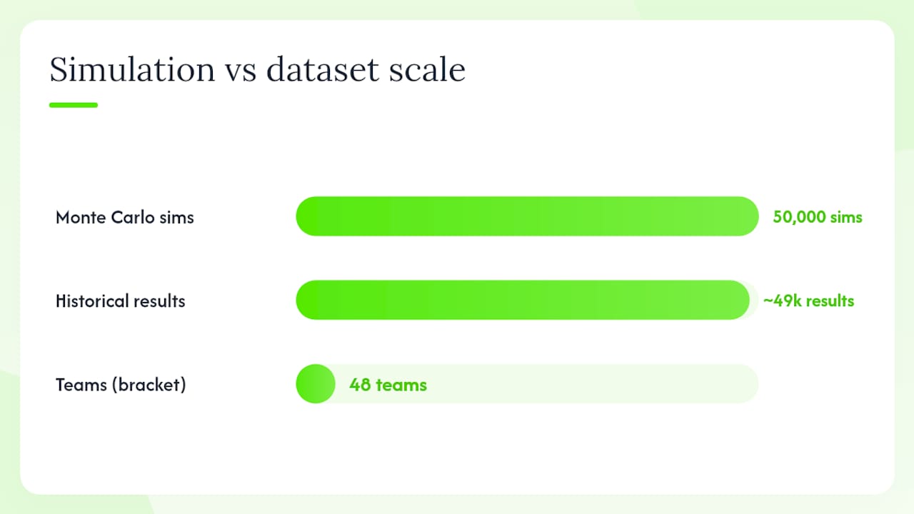
- Hicruben/world-cup-2026-prediction-model: full Elo → Dixon–Coles → Poisson → Monte Carlo pipeline with a live 50,000-simulation example
- Ganapathy-K/fifa-world-cup-2026-forecast: confederation offsets, squad-strength priors (EA Sports FC ratings), and 48-team bracket logic
- jdgoated1/football-predictor: ensemble approach combining Elo, Pi-rating, Dixon–Coles, and ML models (XGBoost/LightGBM) with an isotonic-calibrated meta-learner
- martj42/international_results: the historical match dump (~49,000 results, 1872 to 2026) that most predictors use as core training data
Run a chronological walk-forward backtest first and score it with Brier score, log-loss, and Ranked Probability Score (RPS) before trusting any championship probability output, noting that some backed tests have been done but significance is not guaranteed.
Key Takeaways
The canonical World Cup prediction model pipeline is Elo ratings → Dixon–Coles bivariate Poisson → Monte Carlo simulation (10,000+ runs), validated by chronological walk-forward backtesting scored with Brier, RPS, and log-loss.
| Point | Details |
|---|---|
| Canonical pipeline | Elo → Dixon–Coles bivariate Poisson → Monte Carlo (10k–50k sims) is the reproducible standard. |
| Walk-forward validation | Fit only on pre-match data; score with Brier, RPS, and ECE on a held-out chronological test set. |
| Favorites still lose often | Even the strongest teams carry only ~12–20% championship probability in robust simulation ensembles. |
| Squad priors require care | Use the most recent snapshot on or before each match date to avoid data leakage in squad-prior features. |
| Mannysvariety | Provides production-ready AI-driven soccer picks and daily analytics for bettors who want simulation-backed outputs without building locally. |
Table of Contents
- What do the best open-source World Cup models actually use?
- Which datasets do you need, and how do you clean them?
- How do you convert ratings into scoreline probabilities?
- How do you evaluate a World Cup prediction model honestly?
- How does Monte Carlo simulation turn match odds into tournament forecasts?
- How do you run a baseline model in 30 minutes?
- What are the operational rules for responsible probabilistic forecasting?
- Where do World Cup prediction models commonly fail?
- Why reproducibility and calibration are non-negotiable
- Mannysvariety brings production-ready soccer analytics to your picks
- Sources
What do the best open-source World Cup models actually use?
The canonical building blocks appear in nearly every credible open-source soccer tournament forecasting project:
- Elo or Pi-rating baseline — a time-decayed strength estimate updated after each match result
- Time-decayed attack/defense fits — team-level goal-scoring and conceding rates estimated from recent competitive matches, weighted by recency
- Dixon–Coles bivariate Poisson — the score model that generates full scoreline matrices and corrects the under-representation of 0–0 and 1–1 draws via a correlation term (rho)
- Squad-strength priors — market-value snapshots or EA Sports FC player ratings folded in as a shrinkage target to capture squad quality signals before a tournament begins
- Confederation offsets — adjustments for the different competitive levels across CONMEBOL, UEFA, CONCACAF, AFC, CAF, and OFC
- Monte Carlo simulation — 10,000 to 50,000+ full-tournament runs that aggregate match probabilities into champion and round-progression odds
The white-box vs. black-box trade-off is real. A Dixon–Coles model lets you inspect every coefficient and trace exactly why France is rated 0.3 goals above average in attack. An XGBoost ensemble from jdgoated1/football-predictor may score better on held-out log-loss, but explaining why it assigned a 34% win probability to a given match requires SHAP values and additional tooling. For analysts who need to defend outputs to editors, bettors, or broadcast audiences, the interpretable pipeline usually wins.
Calibration layers sit on top of either approach. Isotonic regression or temperature scaling corrects the overconfidence that complex learners produce, and cnemri/world-cup-2026-predictor documents how central these layers are to producing reliable probabilities rather than well-ranked but poorly calibrated ones.
Engineering extras that matter in practice: venue/host adjustments (the host nation gets a measurable boost), third-place qualifier bracket logic for the 48-team format, and a calibration layer applied after fitting. Skip any one of these and your simulation outputs will drift from observed frequencies.
Which datasets do you need, and how do you clean them?
Primary data sources
The martj42/international_results dataset is the standard starting point: roughly 49,000 international matches from 1872 through 2026, covering results, dates, venues, and tournament types. For squad-strength priors, the two most common sources are Transfermarkt-derived market-value snapshots and EA Sports FC player ratings. The Ganapathy-K forecast uses EA Sports FC 26 ratings (September 2025 snapshot) as an example squad prior.
Preprocessing steps that break reproducibility
Team name canonicalization is the most common silent failure. “USA,” “United States,” and “United States of America” appear as separate teams in raw dumps. Build a name-mapping dictionary before any fitting step.
Neutral venue handling requires a flag on each match. Matches played at neutral sites should not receive a home-advantage adjustment. Many pipelines default every match to home/away and silently inflate home-team ratings.
Time-decay weighting assigns exponentially lower weight to older matches. A half-life of roughly 3–4 years is common for international football, though the exact value should be tuned by leave-one-tournament-out experiments.
Friendly vs. competitive match separation matters. Friendlies carry far less information about true team strength. Most practitioners either exclude them or apply a much lower weight (0.1–0.3 relative to competitive matches).
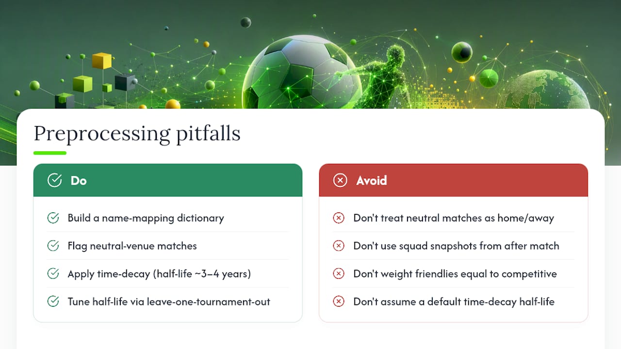
Squad-prior snapshots must be read by match date. Use the most recent snapshot on or before each match date — never a snapshot from after the match. This is the single most common source of data leakage in squad-prior implementations.
Common gotchas
- Data leakage from post-match stats: using final squad values or post-tournament ratings as features for matches that happened before those values were published
- Incorrect 48-team bracket logic: the World Cup 48-team format uses a best-third-placed-team qualification table (Annex C rules) that requires bipartite matching to allocate advancing teams to the correct knockout bracket slots — getting this wrong changes advancement probabilities materially, as documented in the Ganapathy-K forecast
- Inconsistent date/time zones: matches near midnight UTC can appear on the wrong date depending on the source, which breaks chronological train/test splits
| Dataset | Records | Coverage | Primary use |
|---|---|---|---|
| martj42/international_results | ~49,000 matches | 1872–2026 | Core training data for Elo and Dixon–Coles fits |
| EA Sports FC 26 ratings | Per-player ratings | Sept 2025 snapshot | Squad-strength prior for tournament forecasts |
| Transfermarkt market values | Per-squad values | Rolling snapshots | Alternative squad-strength prior |
How do you convert ratings into scoreline probabilities?
Rating baselines
Elo is the most common starting point. The standard Elo update rule adjusts team ratings after each match based on the result and the pre-match expected outcome. Goal-difference-weighted Elo variants (sometimes called “goal Elo”) update ratings more aggressively after large wins, which tends to improve calibration for high-scoring teams. Pi-rating is an alternative that directly models goal difference rather than binary outcomes, and the jdgoated1/football-predictor ensemble includes it alongside Elo as a complementary signal.
Dixon–Coles bivariate Poisson
The Dixon–Coles model fits team-level attack and defense parameters by maximum likelihood over historical scorelines. The key addition over a standard bivariate Poisson is the rho (ρ) correction term, which adjusts the joint probability of 0–0 and 1–1 scorelines upward to match observed draw frequencies. Without rho, the model underestimates low-scoring draws — a meaningful error in international football where 0–0 and 1–1 results are common.
Fitting is done by weighted maximum likelihood, with match weights set by the time-decay function. Numerical stability requires bounding attack and defense parameters away from zero; most implementations clip them at a small positive floor (e.g., 0.01).
Squad-strength priors as shrinkage targets
EA Sports FC ratings or market-value totals enter the model as a Bayesian prior or a shrinkage target on team attack/defense parameters. A team with limited recent match history (a newly promoted qualifier, for example) gets pulled toward its squad-value-implied strength rather than defaulting to a league-average estimate. The prior weight should be tuned by leave-one-tournament-out experiments to avoid overfitting to squad-value signals that don’t translate to match outcomes.
Ensemble options
The jdgoated1/football-predictor ensemble blends Dixon–Coles outputs with XGBoost, LightGBM, and CatBoost classifiers, then stacks them with an isotonic-calibrated logistic meta-learner. The performance gain over a well-tuned Dixon–Coles baseline is modest on held-out international data. The interpretability cost is significant. For most analysts, the white-box baseline is the right starting point; the ensemble is worth adding only after the baseline is validated and calibrated.
How do you evaluate a World Cup prediction model honestly?
Chronological walk-forward backtesting
Fit the model on all matches before a given date, generate predictions for the next block of matches, then advance the window. Never include any information from after the prediction date — not squad values, not tournament results, not updated ratings. The Gwiazdka09/Footstats README documents this as the standard for professional-grade models, and Reymes/football-match-prediction reinforces that strict pre-kickoff feature construction is a design principle, not an optional refinement.
Key metrics
- Brier score: mean squared error between predicted probabilities and binary outcomes; lower is better; a naive 1/3-probability baseline scores around 0.222 for three-outcome football
- Log-loss: penalizes confident wrong predictions more heavily than Brier; useful for detecting overconfidence
- Ranked Probability Score (RPS): accounts for the ordered nature of outcomes (win/draw/loss); preferred for football because it rewards getting the direction right even when the exact outcome is wrong
- Expected Calibration Error (ECE): measures the average gap between predicted probability and observed frequency across probability bins; a well-calibrated model should show ECE below 0.03–0.05
Calibration checks
A perfectly calibrated model produces points on the diagonal. Overconfident models cluster below the diagonal at high probabilities. Isotonic regression or temperature scaling applied post-fit corrects this.
Pro Tip: Use paired block-bootstrap tests against a de-vigged bookmaker closing line to assess whether your model’s edge is statistically significant. Most public models reach parity with closing lines — claiming a sustained edge requires this test, not just a positive log-loss delta on a single tournament.
A careful held-out evaluation often finds public models at parity with de-vigged bookmaker closing lines, as documented in Reymes/football-match-prediction. No public statistical model has conclusively demonstrated a long-term, statistically significant edge over closing lines once rigorous walk-forward tests and paired significance tests are applied, per sinmentis/2026-worldcup-predictor.
How does Monte Carlo simulation turn match odds into tournament forecasts?
Simulation loop design
Each Monte Carlo run simulates the entire tournament from the current state: draw a scoreline for each group-stage match from the Dixon–Coles distribution, determine group standings, apply the best-third-placed-team qualification table, then simulate knockout rounds through to the final. Repeat 10,000 to 50,000 times. The Hicruben/world-cup-2026-prediction-model runs 50,000 simulations; the Ganapathy-K forecast uses 10,000. Both produce stable champion probability estimates — the difference in variance between 10k and 50k runs is small for top teams but noticeable for long-shot qualifiers.
48-team bracket logic
The 2026 World Cup uses 12 groups of 4 teams. The top two from each group advance automatically. Several of the third-placed teams also advance based on standardized criteria across groups. The Annex C rules then determine which knockout bracket slot each advancing third-placed team fills — this requires bipartite matching and cannot be approximated. Implement it exactly or your round-of-32 matchups will be wrong.
Penalty shootouts in knockout rounds are typically modeled as a 50/50 coin flip after a draw, though some implementations use a small home-team or higher-rated-team advantage.
Example simulation outputs
Note: These figures are illustrative of the output format. Run the model against current squad data to generate real probabilities.
Scoreline heatmaps (a matrix of P(home goals = i, away goals = j) for i, j in 0–5) are a useful companion output. They let you read off the most likely exact score, the draw probability, and the tail risk of high-scoring matches.
How do you run a baseline model in 30 minutes?
Recommended repo: Hicruben/world-cup-2026-prediction-model
Step-by-step commands:
git clone https://github.com/Hicruben/world-cup-2026-prediction-modelcd world-cup-2026-prediction-modelpip install -r requirements.txt(requires Python 3.9+, pandas, numpy, scipy, matplotlib)- Place the martj42 results CSV in
data/results.csv python elo_calibration.py— fits Elo ratings and outputs team strength estimatespython match_engine.py— fits Dixon–Coles parameters using time-decayed MLEpython simulation_runner.py --sims 10000— runs 10,000 Monte Carlo tournament simulations- Check
outputs/champion_probabilities.csvandoutputs/calibration_plot.png
Files to inspect:
data/results.csv— confirm team name canonicalization and date coverageelo_calibration.py— adjust the K-factor and time-decay half-life herematch_engine.py— inspect the rho correction and the weighted MLE fitting loopsimulation_runner.py— set--sims,--seed, and--squad_prior_weight
Config knobs to tune first:
--sims: 10,000 for development, 50,000 for final outputs--squad_prior_weight: 0.0 disables the prior; 0.3–0.5 is a reasonable starting range--decay_halflife: time-decay half-life in days (default ~1,000 days; try 800–1,200)
Expected outputs to verify:
- Champion probabilities sum to 100% across all 48 teams
- Calibration plot shows points near the diagonal (not systematically below it)
- No team has a 0% or 100% champion probability unless it has been eliminated
Common errors:
KeyError: team name— team name in results CSV doesn’t match the name mapping dictionary; add the aliasLinAlgErrorduring MLE fitting — attack/defense parameter bounds too loose; tighten the lower bound to 0.01- Simulation probabilities don’t sum to 1.0 — floating-point rounding; normalize the output array
What are the operational rules for responsible probabilistic forecasting?
Caching, seeding, and reproducibility
A production pipeline caches fitted Elo and Dixon–Coles parameters after each fitting run so re-running the simulation doesn’t require re-fitting from scratch. Set a deterministic random seed (numpy.random.seed(42)) and version your data snapshots so any forecast can be reproduced exactly. The Hicruben repo documents this as a core design principle: lock finished matches when running live simulations so completed results don’t get re-simulated.
Common pitfalls
- Leakage from late-arriving features: squad injury reports published after kickoff, final squad lists used for pre-tournament predictions, or post-match ratings used as pre-match features
- Incorrect venue adjustments: applying a home-advantage coefficient to neutral-venue matches inflates the host team’s win probability
- Overfitting to club-level statistics: club form, Champions League performance, and club-level xG don’t transfer cleanly to international football, where squad availability and tactical systems differ significantly
Communicating probabilities to non-technical audiences
The most common mistake is translating a 14% champion probability into “Brazil is the favorite, so they’ll win.” A 100,000-simulation study found that even the strongest favorites carry only ~12–20% championship probability in robust ensembles. Frame outputs as probability distributions, not predictions. For World Cup betting tips, this distinction is the difference between informed wagering and false certainty.
Pro Tip: Run your simulation at 1,000, 5,000, 10,000, and 50,000 iterations and plot champion probability vs. simulation count for the top 5 teams. When the curves flatten (typically around 10,000 runs for top teams, 30,000+ for long shots), you’ve found your minimum viable simulation count.
The interpretability vs. performance trade-off from AI sports betting contexts applies directly here: a model you can explain and audit is worth more in practice than a marginally sharper black box you can’t defend.
Where do World Cup prediction models commonly fail?
The core limitation is tournament variance. A 48-team single-elimination bracket with group-stage randomness produces outcomes that even a perfect probability model cannot predict reliably. The ceiling for any football match prediction model to identify the champion is structurally low.
Known failure modes:
- Cross-confederation calibration: CONMEBOL and UEFA teams play each other rarely outside the World Cup itself, leaving inter-confederation strength estimates poorly anchored. A CONMEBOL team rated 1,700 Elo and a UEFA team rated 1,700 Elo may not be equally strong when they meet.
- Squad availability shocks: a key injury or suspension before a knockout match can shift a team’s true strength by more than any model parameter captures, especially for smaller squads with limited depth
- Tactical adaptation: international managers adjust tactically between matches in ways that historical goal rates don’t capture
- Small sample sizes: most national teams play fewer than 15 competitive matches per year, leaving parameter estimates with wide confidence intervals
Open research questions:
- Better squad-strength priors that integrate positional depth, not just aggregate ratings
- Methods to incorporate off-pitch intelligence (injury reports, lineup confirmations) without introducing leakage
- Reliable approaches to beat de-vigged closing lines consistently — no public model has demonstrated this at statistical significance across multiple tournaments
- Improved cross-confederation calibration using club competition data as a bridge signal
Why reproducibility and calibration are non-negotiable
The open-source repos cited throughout this article share one design principle: every forecast should be reproducible from a fixed data snapshot and a fixed random seed. That’s not a technical nicety. It’s the only way to distinguish a model that genuinely captures signal from one that got lucky on a single tournament.
Walk-forward backtesting is the minimum standard. Any model evaluated on data it was trained on is not a forecast — it’s a memorization exercise. The Brier score, RPS, and ECE metrics only mean something when computed on a held-out chronological test set. Calibration plots only mean something when the bins are populated by out-of-sample predictions.
The same principle applies to probabilistic outputs for bettors. Communicate it that way, track it over hundreds of predictions, and let the calibration plot tell you whether the model is earning its confidence.
Mannysvariety brings production-ready soccer analytics to your picks
Building and validating a World Cup prediction model from scratch takes real time: data cleaning, parameter fitting, bracket logic, calibration checks. Mannysvariety’s AI-powered picks platform runs that analytical work continuously across soccer and multiple other sports, delivering curated picks, player props, and daily reports backed by thousands of simulations and a publicly tracked record of over 1,600 verified picks at a 63.5% win rate and 443.9 units net return.

For analysts who want to study the methodology, the repos above are the right starting point. For bettors who want production-ready outputs without running local Python environments, Mannysvariety’s subscription tiers give you daily intelligence grounded in the same probabilistic framework this article describes. Check pricing and plan options to see which tier fits your workflow.
Mannysvariety is a subscription sports analytics service. Past performance does not guarantee future results. Sports betting involves financial risk; wager responsibly and confirm legality in your jurisdiction.
Sources
The table below covers the primary repos and datasets referenced throughout this article, with notes on what each provides.
- Hicruben/world-cup-2026-prediction-model
- We ran 100,000 computer simulations of the World Cup — and the winner will be…
For probabilistic output communication and the limits of machine-learning forecasts, the AI lottery predictions explainer from Lotto Oracle provides a useful parallel discussion of how probabilistic models should and should not be interpreted by end users.